사이킷런(sklearn)을 이용한 머신러닝 - 3 (군집,분류)

군집을 이해하기 앞서서, 벡터를 이미지를 통해서 이해하시면 편합니다.

%matplotlib inline
import matplotlib.pyplot as plt
import seaborn as sns; sns.set()
import numpy as np
# 이미지를 파일로 출력하고 로딩한다음 글씨만 추출

def make_hello(N=1000, rseed=42):
    fig, ax = plt.subplots(figsize=(4, 1))
    fig.subplots_adjust(left=0, right=1, bottom=0, top=1)
    ax.axis('off')
    ax.text(0.5, 0.4, 'HELLO', va='center', ha='center', weight='bold', size=85)
    fig.savefig('hello.png')
    plt.close(fig)   

    from matplotlib.image import imread
    data = imread('hello.png')[::-1, :, 0].T   
    print("이미지차원", data.shape)
   
    print(data)
    rng = np.random.RandomState(rseed)
    X = rng.rand(4 * N, 2)
    print("만든 갯수",X.shape)
    print((X * data.shape).shape)
    i, j = (X * data.shape).astype(int).T
   
    mask = (data[i, j] < 1)
    X = X[mask]
    print("새로운X갯수", X.shape)
    print("원래이미지의 차수 ", data.shape)
    X[:, 0] *= (data.shape[0] / data.shape[1])
    X = X[:N]

    return X[np.argsort(X[:, 0])]

X = make_hello(1000)
colorize = dict(c=X[:,0], cmap=plt.cm.get_cmap('rainbow',5))

plt.scatter(X[:,0],X[:,1],**colorize)
plt.axis('equal')

이미지차원 (288, 72)
[[1. 1. 1. ... 1. 1. 1.]
 [1. 1. 1. ... 1. 1. 1.]
 [1. 1. 1. ... 1. 1. 1.]
 ...
 [1. 1. 1. ... 1. 1. 1.]
 [1. 1. 1. ... 1. 1. 1.]
 [1. 1. 1. ... 1. 1. 1.]]
만든 갯수 (4000, 2)
(4000, 2)
새로운X갯수 (1532, 2)
원래이미지의 차수  (288, 72)
(-0.11881377209280353,
 4.140158966213945,
 0.02958197717253727,
 1.0142039520339077)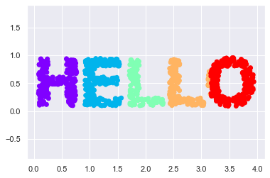

print(X.shape)
def rotate(X, angle):
    theta = np.deg2rad(angle) # 라디안 - 호의 길이
    R = [[np.cos(theta), np.sin(theta)], # 2차원 행열회전
        [-np.sin(theta), np.cos(theta)]]
    print(type(R))
    return np.dot(X,R) #1000*2  2*2 => 1000*2
X2 = rotate(X,20) + 5
plt.scatter(X2[:,0], X2[:,1], **colorize)
plt.axis('equal')

(1000, 2)
<class 'list'>
(4.597858810380142, 8.755757454950324, 5.020644928025307, 7.258448710811383)

# 각 점들간의 상호거리 #디폴트  
from sklearn.metrics import pairwise_distances #  /유클리디안거리
D = pairwise_distances(X) # 거리행렬
print(D.shape)
D[:5,:5]
plt.imshow(D, zorder=2, cmap='Blues', interpolation = 'nearest')
plt.colorbar()

(1000, 1000)
<matplotlib.colorbar.Colorbar at 0x26f465b2788>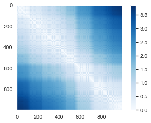

D2 = pairwise_distances(X2)
np.allclose(D,D2) # 원형을 유지하고 있음

True

# 다형체
from sklearn.manifold import MDS
# 미리 계산된 거리행렬을 이용해 차원축소함
# n_components = 2  /2차원
model = MDS(n_components = 2, dissimilarity = 'precomputed', #미리 계산되어진 거리행열
           random_state=1)
out = model.fit_transform(D)
plt.scatter(out[:,0],out[:,1],**colorize)
plt.axis('equal')
print(out)

[[-0.74494191 -1.70588632]
 [-0.41295504 -1.81002158]
 [-0.73486201 -1.70435097]
 ...
 [ 0.75145058  1.84680917]
 [ 0.4906357   1.9307466 ]
 [ 0.63071876  1.89955864]]

고유값 분해

# 고유값 분해
import numpy as np
rng = np.random.RandomState(10)
C = rng.randn(3,3) # normal
print(np.dot(C,C.T)) #전치 행렬, 행렬의 거듭제곱
# 정방행렬 과 대칭행렬이 나옴~~
e,V = np.linalg.eigh(np.dot(C,C.T))
print("eigenvector", V) # 고유벡터
print("eigenvalue", e)# 고유값
np.dot(V[1],V[2]) # 두벡터의 내적 -> 직교

[[4.67300869 1.54608517 0.42456214]
 [1.54608517 0.9046519  0.0621289 ]
 [0.42456214 0.0621289  0.0822976 ]]
eigenvector [[-0.15797077 -0.30570231 -0.93893095]
 [ 0.20981122  0.9187662  -0.33443672]
 [ 0.9648961  -0.24982947 -0.08099843]]
eigenvalue [0.02629875 0.37332691 5.26033253]
-3.122502256758253e-17

 

고유값이란?

[선형대수] 고유값(eigenvalue) 고유벡터(eigenvector)의 의미

def random_projection(X, dimension=3, rseed=42):
    assert dimension >= X.shape[1] # 행,열 (2차원) -> 차원확대만가능
    rng = np.random.RandomState(rseed)
    C = rng.randn(dimension, dimension) # 3*3 
    print("C는", C.shape)
    print(np.dot(C,C.T)) # 정방행열, 대칭
    e,V = np.linalg.eigh(np.dot(C,C.T)) # 고유치와 , 고유벡터
    print("V는", V.shape) # 3*3
    print("차원은", V[:X.shape[1]]) # 2
    return np.dot(X,V[:X.shape[1]]) # 3*2
print(X.shape)
print(X.shape[1])
print("데이터의 차원은", X.shape)
X3 = random_projection(X,3)
X3.shape

(1000, 2)
2
데이터의 차원은 (1000, 2)
C는 (3, 3)
[[0.68534241 0.63723771 0.37423535]
 [0.63723771 2.42926786 2.33541214]
 [0.37423535 2.33541214 3.30327538]]
V는 (3, 3)
차원은 [[-0.63360361  0.75939282  0.14788172]
 [ 0.64803399  0.41652241  0.63762139]]
(1000, 3)

from mpl_toolkits import mplot3d
ax = plt.axes(projection ='3d')
ax.scatter3D(X3[:,0], X3[:,1], X3[:,2],
            **colorize)
ax.view_init(azim=60,elev=30) # azim 좌우로 elev 상하로 카메라다가 보는각도 3차원에서~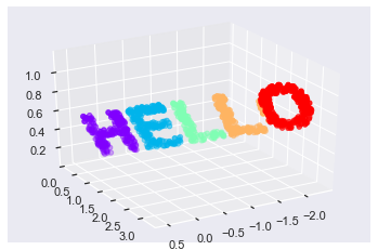

model = MDS(n_components=2, random_state=1)
out3 = model.fit_transform(X3)
plt.scatter(out3[:,0],out3[:,1], **colorize)
plt.axis('equal')

(-1.0390064107727621,
 1.0377133989963219,
 -2.0646660054511297,
 2.135458244484912)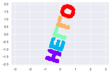

def make_hello_s_curve(X):
    t = (X[:,0]-2) * 0.75 * np.pi
    x = np.sin(t)
    y = X[:,1]
    z = np.sign(t) * (np.cos(t) - 1)
    return np.vstack((x,y,z)).T

XS = make_hello_s_curve(X)
ax = plt.axes(projection='3d')
ax.scatter3D(XS[:,0], XS[:,1],XS[:,2], **colorize)

# MDS 는 비선형에서 모양유지가 안됨
model = MDS(n_components=2, random_state=1)
out3 = model.fit_transform(XS)
plt.scatter(out3[:,0],out3[:,1], **colorize)
plt.axis('equal')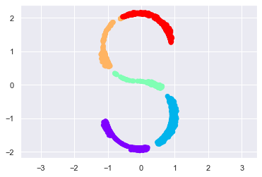

LLE(locally linear embedding)
-비선형에 강함

# 다시 2차원으로 표시
from sklearn.manifold import LocallyLinearEmbedding
model = LocallyLinearEmbedding(n_neighbors=100, n_components =2,
                              method = 'modified', eigen_solver = 'dense')
out = model.fit_transform(XS)
fig, ax = plt.subplots()
ax.scatter(out[:,0], out[:,1], **colorize)
ax.set_ylim(0.15,-0.15)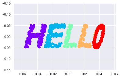

 

---

---

일반적인 분류 문제로 접근방법

import numpy as np
import scipy
import sklearn.metrics.pairwise

a_64 = np.array([61.22,71.60,-65.755], dtype = np.float64)
b_64 = np.array([61.22,71.608,-65.72], dtype = np.float64)
a_32 = a_64.astype(np.float32)
b_32 = b_64.astype(np.float32)
# norm은 원점으로 부터의 크기 ( 단일 벡터 )
dist_64_np = np.array([np.linalg.norm(a_64 -b_64)],
                     dtype = np.float64)
dist_32_np = np.array([np.linalg.norm(a_32 -b_32)],
                     dtype = np.float32)
# euclidean distance 기본값
ist_64_sklearn = sklearn.metrics.pairwise.pairwise_distances([a_64],[b_32], metric = 'manhattan')

from sklearn.svm import SVC # Classifiction 분류
from sklearn.datasets import load_breast_cancer
from sklearn.model_selection import train_test_split
from sklearn.preprocessing import MinMaxScaler #전처리 preprocessing 정규화해서 처리~
# kmeans, PCA 전처리에 민감함
cancer = load_breast_cancer()
X_train, X_test, y_train,y_test = train_test_split(cancer.data, cancer.target, random_state=0)

scaler = MinMaxScaler().fit(X_train) # chaining
X_train_scaled = scaler.transform(X_train)
svm =SVC()
svm.fit(X_train_scaled, y_train)
X_test_scaled = scaler.transform(X_test)
print("테스트점수 : {:.2f}".format(svm.score(X_test_scaled,y_test)))

테스트점수 : 0.95

from sklearn.model_selection import GridSearchCV
from sklearn.svm import SVC
param_grid = {'C' : [0.001, 0.01, 0.1, 1, 10, 100],
             'gamma' : [0.001,0.01,0.1,1,10,100]}
grid = GridSearchCV(SVC(), param_grid=param_grid, cv=5)
grid.fit(X_train_scaled, y_train)
print(" 최상의 교차 검증 정확도 : {:.2f}".format(grid.best_score_))
print("테스트점수: {:.2f}".format(grid.score(X_test_scaled,y_test)))
print("최적의 매개변수: ", grid.best_params_)

최상의 교차 검증 정확도 : 0.98
테스트점수: 0.97
최적의 매개변수:  {'C': 1, 'gamma': 1}

from sklearn.pipeline import Pipeline
from sklearn.preprocessing import MinMaxScaler
# 참조 : 파라미터 전달
pipe = Pipeline([("scaler", MinMaxScaler()), ("svm", SVC())])
pipe.fit(X_train,y_train)
print("train점수: {:.2f}".format(pipe.score(X_test,y_test)))

train점수: 0.95

---

Pipeline+GridSearchCV

# pipeline + GridSearchCV는 다양한 테스트 문제를 해결
from sklearn.model_selection import GridSearchCV
# regularization : 규제 : 과적합을 제하기위해!
from sklearn.svm import SVC
param_grid = {'svm__C' : [0.001, 0.01, 0.1, 1, 10, 100], # 처음엔 대충넣고 최적의 매개변수찾으면 그 수에 맞춰서 세부적으로 나눠서 테스트
             'svm__gamma' : [0.001,0.01,0.1,1,10,100]}
grid = GridSearchCV(pipe, param_grid=param_grid, cv=5)
grid.fit(X_train_scaled, y_train)
print("최상의 교차 검증 정확도 : {:.2f}".format(grid.best_score_))
print("테스트점수: {:.2f}".format(grid.score(X_test_scaled,y_test)))
print("최적의 매개변수: ", grid.best_params_)

최상의 교차 검증 정확도 : 0.98
테스트점수: 0.97
최적의 매개변수:  {'svm__C': 1, 'svm__gamma': 1}

---

군집화 알고리즘 적용전 시각화

한글폰트 사용

import matplotlib.pyplot as plt # 폰트설정
plt.rcParams['font.family'] = 'Malgun Gothic'

 

2차원 도표와 3차원 도표로 시각화

from sklearn.datasets import load_iris
import matplotlib.pyplot as plt
from sklearn import manifold
from matplotlib import pylab
from sklearn.manifold import MDS
from mpl_toolkits import mplot3d
import numpy as np
import os
CHART_DIR = "./"
colors = ['r','g','b']
markers = ["o",6,'*']

def plot_iris_mds():
    iris = load_iris()
    X = iris.data
    y = iris.target
    fig = pylab.figure(figsize=(10, 4))
    ax = fig.add_subplot(121, projection='3d')
    ax.set_facecolor('white')
    mds = manifold.MDS(n_components=3)
    Xtrans = mds.fit_transform(X)
    for cl, color, marker in zip(np.unique(y), colors, markers):
        ax.scatter(
            Xtrans[y == cl][:, 0], Xtrans[y == cl][:, 1], Xtrans[y == cl][:, 2], c=color, marker=marker, edgecolor='black')
    pylab.title("3차원에서 iris MDS")
    ax.view_init(10, -15) # 카메라 각도

    mds = manifold.MDS(n_components=2)
    Xtrans = mds.fit_transform(X)

    ax = fig.add_subplot(122)
    for cl, color, marker in zip(np.unique(y), colors, markers):
        ax.scatter(
            Xtrans[y == cl][:, 0], Xtrans[y == cl][:, 1], c=color, marker=marker, edgecolor='black')
    pylab.title("2차원에서 iris MDS")

    filename = "mds_demo_iris.png"
    pylab.savefig(os.path.join(CHART_DIR, filename), bbox_inches="tight") 

plot_iris_mds()

kmeans : 군집분석 -> 종속변수결정

• 압축 : 팔레트 , 실제데이터에는 팔레트 번호를 넣어서 한번 참조함(256) = 1byte로 표현이가능
• 원형이상치 제거
• 미리 군집화해서 문제해결에 도움을 줌

  알고리즘 - k값을 결정 (군집수결정), 중심값 : 중심이 변화(재계산)

• 문제점 : 이상치에 민감

  kmeans의 척도 : 거리값 (피타고라스 정리 -> euclidian distance)

  DBSCAN : eps 기본 거리값, 군집이 되기 위한 최소요소수

• 핵심, 경계, 어느 군집에도 속하지 않는 것 / 총 3개로 나눠짐

---

K-means 군집화

# 초기 중심값이 결정 입력 => 중심은 지속적으로 변화됨~
# 중심과의 거리값  /거리값이 멀어있으면 문제임
from sklearn import cluster, datasets
import matplotlib.pyplot as plt
import seaborn as sns
%matplotlib inline
iris = datasets.load_iris()
X = iris.data[:,:2] # 전체변수 4 -> 2개
y_iris = iris.target
km2 = cluster.KMeans(n_clusters=2).fit(X)
km3 = cluster.KMeans(n_clusters=3).fit(X)
km4 = cluster.KMeans(n_clusters=4).fit(X)
plt.figure(figsize=(9,3)); plt.subplot(131)
plt.scatter(X[: ,0], X[:,1],c=km2.labels_) # 컬러 2
plt.title("K=2, J=%.2f" % km2.inertia_) #군집 내부 거리값
# inertia = 중심점으로부터의 거리제곱의 합
plt.subplot(132); plt.scatter(X[:,0],X[:,1],c=km3.labels_)
plt.title("K=3, J=%.2f" % km3.inertia_)
plt.subplot(133); plt.scatter(X[:,0],X[:,1],c=km4.labels_)
plt.title("K=3, J=%.2f" % km4.inertia_)
km4.cluster_centers_ # 중심값

array([[6.91025641, 3.08717949],
       [4.76666667, 2.89166667],
       [5.1875    , 3.6375    ],
       [5.93818182, 2.77090909]])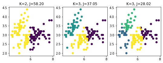

km4.cluster_centers_ # 중심값 !!

array([[4.76666667, 2.89166667],
       [6.91025641, 3.08717949],
       [5.1875    , 3.6375    ],
       [5.93818182, 2.77090909]])

X = np.array([[7,5],[5,7],[7,7],[4,4],[4,6],[1,4],
             [0,0],[2,2],[8,7],[6,8],[5,5],[3,7]])
plt.scatter(X[:,0],X[:,1],s=100)
plt.show()

from sklearn.cluster import KMeans
# 레이블 : 군집번호 : 종속변수
model = KMeans(n_clusters=2, init ="random", n_init=1, max_iter=1,random_state=1).fit(X)
c0,c1 = model.cluster_centers_
print(len(model.labels_))
# boolean index / label이 0인것만 찾아라~ true니깐~
plt.scatter(X[model.labels_==0,0], X[model.labels_==0,1], s=100,
           marker ='v', c='r')
plt.scatter(X[model.labels_==1,0], X[model.labels_==1,1], s=100,
           marker ='^', c='b')
plt.scatter(c0[0], c0[1], s=100, c="r")
plt.scatter(c1[0], c1[1], s=100, c="b")
plt.show()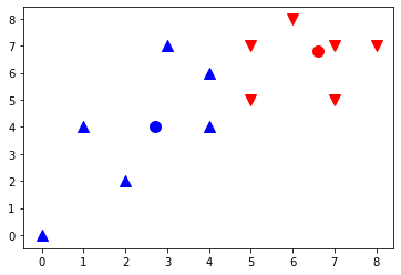

---

IMAGE 변형 및 출력

from sklearn.datasets import load_sample_image
from sklearn.utils import shuffle
from time import time
import numpy as np
from sklearn.cluster import KMeans
import matplotlib.pyplot as plt

from matplotlib import font_manager, rc
font_name=font_manager.FontProperties(fname="c:/Windows/Fonts/malgun.ttf").get_name()
rc('font', family =font_name)

n_color = 64
# 1바이트 = 8비트 =표현종류 -> 256가지~
china = load_sample_image("flower.jpg") # RGB
# 컬러값 정규화 0~1정규화
china = np.array(china, dtype=np.float64)/255

w, h, d = original_shape = tuple(china.shape) # 이미지 행*열, 3
print(w, h ,d)
assert d == 3 # RGB만 들어와라~
image_array = np.reshape(china, (w*h,d)) # 2차원으로

427 640 3

# 1000개의 행
image_array_sample = shuffle(image_array, random_state = 0)[:1000]
# 64컬러로 군집화
kmeans = KMeans(n_clusters=n_color, random_state=0).fit(image_array_sample) #중심값 결정 64개

labels = kmeans.predict(image_array) # 라벨

def recreate_image(codebook, labels, w, h): # codebook은 64컬러값, labels=이미지픽셀값
    d = codebook.shape[1] # 64 개의 중심값  64*3
    image = np.zeros((w,h,d)) # 원래 이미지 사이즈
    label_idx = 0
    for i in range(w):
        for j in range(h):
            image[i][j] = codebook[labels[label_idx]]
            label_idx += 1
    return image

plt.figure(1)
plt.clf()
ax = plt.axes([0,0,1,1])
plt.axis('off')
plt.title('Original 이미지 (96,615 colors)')
plt.imshow(china)
plt.figure(2)
plt.clf()
ax = plt.axes([0,0,1,1])
plt.axis('off')
plt.title('64컬러 이미지 (64 colors)')
plt.imshow(recreate_image(kmeans.cluster_centers_, labels,w,h))

 

 

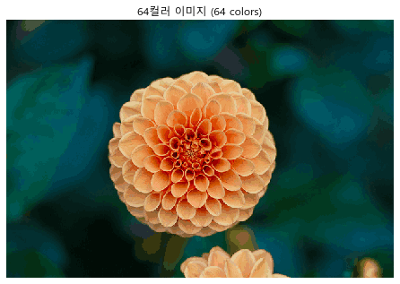
image = plt.imread("12.jpg")
plt.figure(figsize=(15,8))
plt.imshow(image)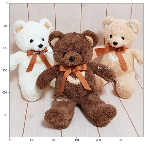

# 바이트수
image.shape[0] * image.shape[1] * image.shape[2]

1080000

from sklearn import cluster
x,y,z = image.shape
image = np.array(image, dtype = np.float64) / 255
image_2d = image.reshape(x*y,z) # kmeans는 3차원을 이해하지못함! 2차원만
image_2d.shape

(360000, 3)

 

kmeans_cluster = cluster.KMeans(n_clusters=16)
kmeans_cluster.fit(image_2d)
cluster_centers = kmeans_cluster.cluster_centers_
cluster_centers

array([[0.78473247, 0.47317372, 0.30351544],
       [0.84288605, 0.81108996, 0.80022472],
       [0.31903211, 0.15168343, 0.0982614 ],
       [0.70838233, 0.57325506, 0.4896986 ],
       [0.47825228, 0.30501312, 0.23548539],
       [0.87353566, 0.85254756, 0.84379605],
       [0.19208189, 0.05968307, 0.03218445],
       [0.91712561, 0.93025912, 0.92216596],
       [0.55571942, 0.38213999, 0.30533291],
       [0.8098051 , 0.77232848, 0.75350092],
       [0.85578356, 0.74693555, 0.64905935],
       [0.6397032 , 0.30081173, 0.16652482],
       [0.40536151, 0.22981003, 0.16676673],
       [0.63352125, 0.47068571, 0.38875016],
       [0.90558005, 0.82081983, 0.73796522],
       [0.77531979, 0.66563638, 0.58366567]])

len(cluster_centers)

16

cluster_centers.shape

(16, 3)

 

cluster_labels = kmeans_cluster.labels_
cluster_labels

array([9, 9, 9, ..., 5, 5, 5])

plt.figure(figsize = (15,8))
plt.imshow(cluster_centers[cluster_labels].reshape(x,y,z))

---

원형 이상치 제거

from sklearn.datasets import make_blobs
X, label = make_blobs(100, centers = 1)

kmeans = KMeans(n_clusters=1) # 중심 1개
kmeans.fit(X)
distances = kmeans.transform(X) # 각 데이터의 중심으로 부터 값으로 변환
# ravel() 1차원으로 만들때 ~
# argsort = 인덱스를 sort해라 ~ 이값으로 다른값을 컨트롤 하고싶어서~
# 2개가
# 내림차순으로 변경
# [::-1] 꺼꾸로~
sorted_idx = np.argsort(distances.ravel())[::-1][:5]

f, ax = plt.subplots(figsize =(7,5))
ax.set_title('Single Cluster')
ax.scatter(X[:,0],X[:,1],label = 'Points')
ax.scatter(kmeans.cluster_centers_[:,0],
        kmeans.cluster_centers_[:,1],
          label = 'Centroid', color = 'r')
ax.scatter(X[sorted_idx][:,0],
          X[sorted_idx][:,1],
          label='이상치', edgecolors='g',
          facecolors='none',s=100)
ax.legend(loc='best')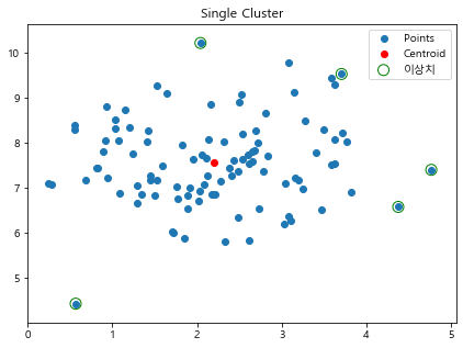

---

PCA(차원축소)

# PCA : Principle component Analysis
# 모델 입력 전단에서 특징 추출 (noise 제거)
# PCA의 결과를 모델의 변수로 추가하면 정확도가 상승해서 ***
import numpy as np
from sklearn.decomposition import PCA
X = np.array([[-1,-1],[-2,-1],[-3,-2],[1,1],[2,1],[3,2]])
pca = PCA(n_components=2) # 주성분을 2개로 해라~
pca.fit(X)
print(pca.explained_variance_ratio_) # 설명력!! 중요~ / 축이름을 재명령 해야함~

[0.99244289 0.00755711]

차원축소후에 분석을 하면 좋은점

• noise 제거
• 속도가 개선
• 차원의 저주(차원이 많으면 복잡해서;;) -> 복잡한 문제를 해결

print(pca.explained_variance_) # 분산이 큰것이 주성분~~!
print(pca.noise_variance_) # Noise

[7.93954312 0.06045688]
0.0

 

svd 희소행렬 특징추출
500*500 이면 사용 = randomized
arpack = 0을 없애서 출력

pca = PCA(n_components=2, svd_solver='full') # singular value decomposition

pca.fit(X)
print(pca.explained_variance_ratio_)

[0.99244289 0.00755711]

from sklearn.datasets import load_breast_cancer
from sklearn.model_selection import train_test_split
cancer = load_breast_cancer()
X_train, X_test, y_train,y_test = train_test_split(cancer.data, cancer.target, random_state=0)

print(type(X_train))
print(X_train.shape)
print(X_train.dtype)
print(X_test.shape)

<class 'numpy.ndarray'>
(426, 30)
float64
(143, 30)

---

SVM 모델을 사용하기전 Scale의 한것과 안한것의 차이

# scaler 안한거~
from sklearn.svm import SVC
svm = SVC(C=100)
svm.fit(X_train, y_train)
print("테스트 세트 정확도:{:.2f}".format(svm.score(X_test,y_test)))

테스트 세트 정확도:0.63

 

MinMax scale 사용

# scaler한거~
from sklearn.preprocessing import MinMaxScaler
scaler = MinMaxScaler()
scaler.fit(X_train)
X_train_scaled = scaler.transform(X_train)
X_test_scaled = scaler.transform(X_test)
svm.fit(X_train_scaled, y_train)
print("스케일 조정된 테스트 세트의 정확도: {:.2f}".format(svm.score(X_test_scaled,y_test)))

스케일 조정된 테스트 세트의 정확도: 0.97

 

StandardScale 사용(정규분포로 변환)

from sklearn.preprocessing import StandardScaler
cancer = load_breast_cancer()
scaler = StandardScaler()
scaler.fit(cancer.data)
X_scaled = scaler.transform(cancer.data)

스케일 조정된 상태에서 PCA 진행

pca = PCA(n_components = 18)
pca.fit(X_scaled)
# 2개의 주성분을 출력
X_pca = pca.transform(X_scaled)
print(pca.explained_variance_ratio_)
# 569,30 / 28개의 특성을 제거~
print("원본데이터 형태 : {}".format(str(X_scaled.shape)))
print("축소된 데이터 형태 : {}".format(str(X_pca.shape)))
plt.plot(np.cumsum(pca.explained_variance_ratio_))

[0.44272026 0.18971182 0.09393163 0.06602135 0.05495768 0.04024522
 0.02250734 0.01588724 0.01389649 0.01168978 0.00979719 0.00870538
 0.00804525 0.00523366 0.00313783 0.00266209 0.00197997 0.00175396]
원본데이터 형태 : (569, 30)
축소된 데이터 형태 : (569, 18)

plt.plot(pca.explained_variance_ratio_, 'bo-')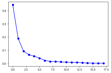

최종적으로 StandardScale을 이용해서 정규화를 진행하고,

그다음 PCA를 이용해 차원을 축소해서 SVM 머신러닝 모델을 생성했습니다.

# 매우중요함~!!
from sklearn.preprocessing import StandardScaler
from sklearn.decomposition import PCA

scaler = StandardScaler() # 정규화 z 점수~
scaler.fit(X_train)
X_train_scaled = scaler.transform(X_train)
X_test_scaled = scaler.transform(X_test)

pca = PCA(n_components=6) # 전체 변수 30개
pca.fit(X_train_scaled)
X_t_train = pca.transform(X_train_scaled)
X_t_test = pca.transform(X_test_scaled)
svm.fit(X_t_train, y_train)
print("SVM 테스트 정확도: {:.2f}".format(svm.score(X_t_test,y_test)))

# 6 : 97%
# 9 : 97%

SVM 테스트 정확도: 0.97

print("PCA 주성분 형태: {}".format(pca.components_.shape))
# 6,30 주성분을 60개의 변수가 설명 -> 주성분 축 : 명명
# 변수의 기여도를 보고 명명식

PCA 주성분 형태: (6, 30)

 

print("PCA 주성분 : {}".format(pca.components_))

PCA 주성분 : [[ 2.21365239e-01  1.00002186e-01  2.29518109e-01  2.23520981e-01
   1.43022884e-01  2.42110713e-01  2.60269250e-01  2.64252721e-01
   1.34215403e-01  5.85049993e-02  2.06864788e-01  7.29622255e-03
   2.09874216e-01  2.02238408e-01  1.72518718e-02  1.66390255e-01
   1.38559209e-01  1.79940925e-01  2.94390431e-02  1.01929667e-01
   2.30419562e-01  1.00571999e-01  2.37796607e-01  2.27510089e-01
   1.31359787e-01  2.10778835e-01  2.30141898e-01  2.53344062e-01
   1.19116509e-01  1.30882592e-01]
 [-2.30173200e-01 -5.72175515e-02 -2.13355030e-01 -2.26935339e-01
   1.78770408e-01  1.47448613e-01  6.55746283e-02 -3.13406669e-02
   1.90507115e-01  3.63961224e-01 -1.05013647e-01  9.39735986e-02
  -9.74743957e-02 -1.49610324e-01  2.12040027e-01  2.35434997e-01
   2.10509206e-01  1.52280137e-01  1.81074900e-01  2.78679424e-01
  -2.15982904e-01 -4.24949684e-02 -2.00035990e-01 -2.15181923e-01
   1.71468563e-01  1.38831730e-01  1.05033622e-01  6.40329376e-04
   1.40657666e-01  2.73186544e-01]
 [-5.09146639e-03  2.95219102e-02 -5.35984824e-03  3.64872826e-02
  -9.76061178e-02 -7.56281849e-02  2.25777028e-02 -1.69771209e-02
  -3.70078138e-02 -2.54673100e-02  2.80308925e-01  3.48764868e-01
   2.74210163e-01  2.32685298e-01  2.94564117e-01  1.59979107e-01
   1.91332037e-01  2.12032925e-01  2.88011717e-01  2.12034692e-01
  -4.64343464e-02 -8.28480024e-02 -4.63440319e-02 -6.32639693e-03
  -2.64083982e-01 -2.45597219e-01 -1.63048941e-01 -1.74418762e-01
  -2.73132934e-01 -2.35424811e-01]
 [-5.09750137e-02  6.09643449e-01 -5.05442992e-02 -5.19396959e-02
  -9.90956857e-02 -3.43388160e-02 -2.03792551e-02 -4.85682624e-02
  -4.82936670e-02 -3.33058678e-02 -5.61443640e-02  4.09044347e-01
  -5.41910430e-02 -7.10889232e-02  2.28841721e-02  4.04038956e-03
  -3.48240995e-02 -8.96070976e-02 -4.47157568e-02 -2.73515484e-02
  -1.63694522e-02  6.34748740e-01 -1.69618164e-02 -1.44718484e-02
   3.18140229e-02  5.49674834e-02  4.24308399e-02 -1.88766860e-02
   9.67337668e-03  4.82147608e-02]
 [ 2.91674793e-02  1.63422384e-02  2.87254429e-02 -8.79337712e-05
  -3.87189925e-01  9.00146532e-04  9.13549118e-02 -4.92250615e-02
  -2.90281096e-01 -5.56708996e-02 -1.59698300e-01 -1.34902267e-01
  -1.34796845e-01 -1.41007648e-01 -2.75448115e-01  2.71368637e-01
   3.61360912e-01  2.02067692e-01 -2.67865520e-01  2.52035781e-01
  -1.37950482e-03 -1.26066877e-02  6.91797569e-03 -2.52811454e-02
  -3.13514426e-01  1.12234403e-01  2.01152630e-01  4.44252770e-02
  -2.26149739e-01  8.20881806e-02]
 [ 1.95382098e-02  3.35010358e-02  1.55094885e-02 -3.06876780e-03
  -2.93046725e-01 -3.36569227e-02 -1.54231618e-02 -4.92546020e-02
   3.79266059e-01 -1.43907450e-01 -2.65867058e-02 -3.18141309e-02
  -2.33390764e-02 -5.69970898e-02 -2.97493845e-01  6.05385639e-02
   4.71977007e-02 -1.98387425e-02  4.83927792e-01 -2.99046124e-02
   9.89299672e-03  3.41203682e-03  1.25825935e-02 -1.80108943e-02
  -3.48935668e-01  3.72397718e-02  2.27132909e-02 -1.34670780e-02
   5.26499723e-01 -8.36959074e-02]]

plt.matshow(pca.components_, cmap='viridis')
plt.colorbar()

---

이미지를 이용한 주성분 분석

%matplotlib inline
from sklearn.datasets import fetch_lfw_people
import matplotlib.pyplot as plt
people = fetch_lfw_people(min_faces_per_person=20, resize=0.7)
image_shape = people.images[0].shape
print(image_shape) # 87*65 , 이미지를 가로x세로, 행렬 행부터
fig, axes = plt.subplots(2,5,figsize = (15,8),
                        subplot_kw={'xticks': (), 'yticks': ()})
for target, image, ax in zip(people.target, people.images,
                            axes.ravel()):
    ax.imshow(image)
    ax.set_title(people.target_names[target])

print("이미지사이즈 :{}".format(people.images.shape))
print("클래스 개수: {}".format(len(people.target_names)))

이미지사이즈 :(3023, 87, 65)
클래스 개수: 62

mask = np.zeros(people.target.shape,dtype=np.bool)
for target in np.unique(people.target):
    mask[np.where(people.target == target)[0][:50]] = 1
X_people = people.data[mask]
y_people = people.target[mask]
X_poeple = X_people/255.

X_train, X_test, y_train, y_test = train_test_split(X_people,y_people,stratify=y_people, random_state=0)

from sklearn.decomposition import PCA
pca = PCA(n_components = 100, whiten=True, random_state=0).fit(X_train)
X_train_pca = pca.transform(X_train)
X_test_pca = pca.transform(X_test)

fig, axes = plt.subplots(3,5, figsize=(15,12), subplot_kw={'xticks' : (), 'yticks' : ()})
for i, (component, ax) in enumerate(zip(pca.components_,axes.ravel())):
    ax.imshow(component.reshape(image_shape), cmap='viridis')
    ax.set_title("주성분{}".format((i+1)))

컴퓨터가 주성분분석을 통해 찾아낸 주성분
100개를 합하여 출력 원본이미지를 복원 -> ANN 의 가중치 특징을 설명할 수 없습니다..